Decoding a Black Hole: From Scrambling to Information Loss¶
Hayden-Preskill Thought Experiment + Yoshida-Kitaev Protocol¶
1. Information Loss Puzzle¶
Fundamental Conflict Between Quantum Mechanics and General Relativity¶
Quantum mechanics states: Information is never lost
$$|\psi(t)\rangle = e^{-i\hat{H}t/\hbar}|\psi(0)\rangle$$
Unitary evolution preserves information - any quantum process is in principle reversible.
General relativity suggests: Information falling into a black hole is lost forever
- Black holes emit thermal Hawking radiation
- After complete evaporation of the black hole, all information should vanish
- This would violate unitarity of quantum mechanics
2. Hayden-Preskill Thought Experiment (2007)¶
Basic Setup¶
Protagonists:
- Alice: owns a quantum state |ψ⟩ that she wants to send into the black hole
- Bob: owns a quantum memory M that is maximally entangled with the black hole
Scenario:
- The black hole has already radiated ~50% of its content (reached Page time)
- At this moment, the black hole is maximally entangled with the previous Hawking radiation
- Bob collects this radiation and maintains it in his quantum memory M
Key Finding:
After Page time, information begins to leak out rapidly from the black hole through Hawking radiation!
Two Types of Black Holes¶
A) Evaporating Black Hole¶
- Starts with a large amount of mass
- Gradually emits Hawking radiation
- After radiating ~50% of content, reaches Page time
- Continues evaporating until complete disappearance
B) Eternal AdS Black Hole (eternal black hole in Anti-de Sitter space)¶
- Maintains constant size
- In thermal equilibrium with its radiation
- Described by the thermofield double state
- This model is more suitable for quantum experiments
3. Simulation of the black hole information paradox¶
Circuit structure:¶
- q0: falling qubit carrying unknown information
- q1-q4: black hole that entangle the information
- q5: external reference qubit that remains outside the black hole
- q6: used for collecting qubits emitted as Hawking radiation
- q7: used for verifying quantum correlations
- After scrambling, we gradually "emit" qubits as Hawking radiation
from qiskit import QuantumCircuit, QuantumRegister, ClassicalRegister
from qiskit.quantum_info import DensityMatrix, partial_trace, entropy
from qiskit_aer import AerSimulator
from qiskit import transpile
import numpy as np
import matplotlib.pyplot as plt
from scrambling_circuit import ScramblingCircuit

m_rnd_value = 80
scramble_depth = 4
%matplotlib inline
np.random.seed(m_rnd_value)
4. Circuits¶
def hp_circuit1():
    qr = QuantumRegister(8, 'q')
    cr = ClassicalRegister(2, 'c')
    qc = QuantumCircuit(qr, cr)
    qc.h(qr[5])
    qc.h(qr[7])
    qc.cx(qr[5], qr[0])
    qc.cz(qr[0], qr[5])
    qc.barrier(label='Bell A↔R')
    qc.h(qr[0])
    qc.barrier(label='BH init')

    qc.cx(qr[0], qr[1])
    qc.cx(qr[0], qr[2])
    qc.cx(qr[0], qr[3])
    qc.cx(qr[0], qr[4])
    qc.barrier(label='q0→BH')

    # === Scrambling - systematic CNOT cascades ===
    for source in range(5):
        for target in range(5):
            if source != target:
                qc.cx(qr[source], qr[target])
    for i in range(5):
        qc.rx(np.random.uniform(0, 2*np.pi), qr[i])
        qc.ry(np.random.uniform(0, 2*np.pi), qr[i])
        qc.rz(np.random.uniform(0, 2*np.pi), qr[i])

    qc.barrier(label='Scramble')

    qc.cx(qr[2], qr[6])
    qc.cx(qr[3], qr[6])
    qc.cx(qr[4], qr[6])

    qc.h(qr[6])

    qc.cswap(qr[7],qr[6],qr[5])

    qc.h(qr[7])
    qc.barrier(label='Radiation→q6')

    return qc, qr, cr

def hp_circuit2(scramble_depth=scramble_depth):
    """
    Hayden-Preskill circuit.
    """
    qr = QuantumRegister(8, 'q')
    cr = ClassicalRegister(2, 'c')
    qc = QuantumCircuit(qr, cr)

    # ========== 1. Bell pair: q0 (falling) ↔ q5 (reference) ==========
    # |Φ+⟩ = (|00⟩ + |11⟩)/√2
    # q5 stays OUTSIDE as reference
    qc.h(qr[5])
    qc.h(qr[7])
    qc.cx(qr[5], qr[0])
    qc.cz(qr[0], qr[5])
    qc.barrier(label='Bell q0↔q5')

    # ========== 2. Black hole (q1-q4) in initial state ==========
    # We can initialize as maximally mixed state
    qc.h(qr[0])
    #for i in range(0, 5):  # q1-q4
    #    qc.h(qr[i])
    #for i in range(0, 5):
    #    qc.h(qr[i])
    qc.barrier(label='BH init')

    # ========== 3. q0 falls into the black hole ==========
    # Interaction of falling qubit with BH qubits
    for i in range(1, 5):
        qc.cx(qr[0], qr[i])
    qc.barrier(label='q0→BH')

    # ========== 4. Scrambling inside the black hole ==========
    for layer in range(scramble_depth):
        # Random single-qubit rotations on BH (q0-q4)
        for i in range(5):
            qc.rx(np.random.uniform(0, 2*np.pi), qr[i])
            qc.ry(np.random.uniform(0, 2*np.pi), qr[i])
            qc.rz(np.random.uniform(0, 2*np.pi), qr[i])
        # CNOT layer (forward) - only within BH
        for i in range(4):
            qc.cx(qr[i], qr[i+1])
        # CNOT layer (backward)
        for i in range(3, -1, -1):
            qc.cx(qr[i+1], qr[i])
    qc.barrier(label='Scramble')

    # ========== 5. Hawking radiation emission to q6 ==========
    # Qubits from BH (q1, q2, q3) radiate information to q6
    #qc.cx(qr[1], qr[6])
    qc.cx(qr[2], qr[6])
    qc.cx(qr[3], qr[6])
    qc.cx(qr[4], qr[6])
    qc.h(qr[6])

    qc.cswap(qr[7],qr[6],qr[5])

    qc.h(qr[7])
    qc.barrier(label='Radiation→q6')
    return qc, qr, cr
5a. Visualisation circuits¶
qc, qr, cr = hp_circuit1()
qc.draw(output='mpl', fold=80, scale=0.6)

5b. Visualisation circuits¶
qc, qr, cr = hp_circuit2(scramble_depth=scramble_depth)
qc.draw(output='mpl', fold=80, scale=0.6)

6a. Analysis: Mutual Information vs Number of Emitted Qubits¶
def analyze_emission(qc, n_emitted):
    """
    Modified analysis for correct qubit structure:
    - q0: falling qubit (in BH)
    - q1-q4: black hole
    - q5: REFERENCE - Bell pair with q0
    - q6: Hawking radiation
    - q7: SWAP test (not used here)

    Emission: we gradually "radiate" qubits from BH (q0, q1, q2, q3, q4)
    """
    sim = AerSimulator(method='statevector')
    qc_copy = qc.copy()
    qc_copy.save_statevector()
    result = sim.run(transpile(qc_copy, sim)).result()
    rho = DensityMatrix(result.get_statevector())

    all_q = set(range(8))
    ref = [5]

    # Radiation = first n_emitted qubits from BH (q0, q1, ...)
    rad = list(range(n_emitted)) if n_emitted > 0 else []

    # BH remainder = from n_emitted to q4 (total 5 BH qubits: q0-q4)
    bh = list(range(n_emitted, 5))

    def S(sub):
        if not sub:
            return 0.0
        return entropy(partial_trace(rho, list(all_q - set(sub))), base=2)

    def MI(A, B):
        if not A or not B:
            return 0.0
        return S(A) + S(B) - S(list(set(A) | set(B)))

    return {
        'n_emitted': n_emitted,
        'fraction': n_emitted / 5,  # 5 qubits in BH
        'I(R:Rad)': MI(ref, rad),
        'I(R:BH)': MI(ref, bh),
        'S(R)': S(ref),
        'S(Rad)': S(rad),
        'S(BH)': S(bh),
    }
qc_full, qr, cr = hp_circuit1()
# Analysis for different numbers of emitted qubits
results = []
for n in range(7):
    res = analyze_emission(qc_full, n)
    results.append(res)
print(f"S(Reference) = {results[0]['S(R)']:.4f} bits\n")
print("Emitted   | Fraction |  I(R:Rad)  |  I(R:BH)  |  S(Rad)  |  S(BH)")
print("-" * 70)
for res in results:
    marker = " ← Page time" if res['n_emitted'] == 3 else ""
    print(f"    {res['n_emitted']}     |  {res['fraction']:.2f}   |   {res['I(R:Rad)']:.4f}   |  {res['I(R:BH)']:.4f}  |  {res['S(Rad)']:.4f}  |  {res['S(BH)']:.4f}{marker}")
S(Reference) = 1.0000 bits

Emitted   | Fraction |  I(R:Rad)  |  I(R:BH)  |  S(Rad)  |  S(BH)
----------------------------------------------------------------------
    0     |  0.00   |   0.0000   |  1.1887  |  0.0000  |  2.0000
    1     |  0.20   |   0.4512   |  0.4512  |  1.0000  |  1.0000
    2     |  0.40   |   0.4512   |  0.4512  |  1.0000  |  1.0000
    3     |  0.60   |   0.7736   |  0.1917  |  1.9908  |  0.9994 ← Page time
    4     |  0.80   |   0.7754   |  0.1899  |  1.9957  |  0.9987
    5     |  1.00   |   1.1887   |  0.0000  |  2.0000  |  0.0000
    6     |  1.20   |   1.0000   |  0.0000  |  1.8113  |  0.0000
7a. Visualisation: Page curve¶
fig, axes = plt.subplots(1, 3, figsize=(15, 5))
fig.suptitle('Hayden-Preskill Protocol: Information Escaping', fontsize=14, fontweight='bold')
n_emit = [r['n_emitted'] for r in results]
fracs = [r['fraction'] for r in results]
I_rad = [r['I(R:Rad)'] for r in results]
I_bh = [r['I(R:BH)'] for r in results]
S_rad = [r['S(Rad)'] for r in results]
# 1. Mutual Information
ax1 = axes[0]
ax1.plot(n_emit, I_rad, 'b-o', lw=2, ms=10, label='I(Reference : Radiation)')
ax1.plot(n_emit, I_bh, 'r--s', lw=2, ms=8, label='I(Reference : BH)')
ax1.axvline(x=3, color='green', linestyle=':', lw=2, alpha=0.7, label='Page time')
ax1.set_xlabel('Number of emitted qubits', fontsize=11)
ax1.set_ylabel('Mutual Information [bits]', fontsize=11)
ax1.set_title('Where does information escape to?')
ax1.legend(loc='center right')
ax1.grid(True, alpha=0.3)
ax1.set_xticks(n_emit)
# 2. Page curve - S(Radiation)
ax2 = axes[1]
ax2.plot(n_emit, S_rad, 'm-^', lw=2, ms=10, label='S(Radiation)')
# Theoretical Page curve
page_theory = [min(k, 6-k) for k in range(7)]
ax2.plot(n_emit, page_theory, 'g--', lw=2, alpha=0.5, label='Page curve (ideal)')
ax2.axvline(x=3, color='green', linestyle=':', lw=2, alpha=0.7)
ax2.set_xlabel('Number of emitted qubits', fontsize=11)
ax2.set_ylabel('Entropy [bits]', fontsize=11)
ax2.set_title('Page Curve')
ax2.legend()
ax2.grid(True, alpha=0.3)
ax2.set_xticks(n_emit)
# 3. Information fraction in radiation
ax3 = axes[2]
total = [r + b for r, b in zip(I_rad, I_bh)]
ratio = [r/t*100 if t > 0.01 else 0 for r, t in zip(I_rad, total)]
colors = ['#2196F3' if r < 50 else '#4CAF50' for r in ratio]
ax3.bar(n_emit, ratio, color=colors, edgecolor='black', alpha=0.8)
ax3.axhline(y=50, color='red', linestyle='--', lw=2, alpha=0.7, label='50% threshold')
ax3.axvline(x=3, color='green', linestyle=':', lw=2, alpha=0.7, label='Page time')
ax3.set_xlabel('Number of emitted qubits', fontsize=11)
ax3.set_ylabel('Information fraction in radiation [%]', fontsize=11)
ax3.set_title('Decodability from radiation')
ax3.set_ylim(0, 110)
ax3.legend()
ax3.grid(True, alpha=0.3)
ax3.set_xticks(n_emit)
plt.tight_layout()
plt.show()

8a. Statistics across different scrambling realizations¶
def run_multiple_realizations(n_realizations=5, scramble_depth=scramble_depth, m_rnd_value=m_rnd_value):
    """Averages over different random scrambling unitaries."""
    all_I_rad = []
    all_I_bh = []

    for seed in range(n_realizations):
        np.random.seed(seed * 17 + m_rnd_value)
        qc, _, _ = hp_circuit1()

        I_rad_run = []
        I_bh_run = []
        for n in range(7):
            res = analyze_emission(qc, n)
            I_rad_run.append(res['I(R:Rad)'])
            I_bh_run.append(res['I(R:BH)'])

        all_I_rad.append(I_rad_run)
        all_I_bh.append(I_bh_run)

    return {
        'mean_I_rad': np.mean(all_I_rad, axis=0),
        'std_I_rad': np.std(all_I_rad, axis=0),
        'mean_I_bh': np.mean(all_I_bh, axis=0),
        'std_I_bh': np.std(all_I_bh, axis=0),
    }

stats = run_multiple_realizations(n_realizations=5)
print("Emitted   |  I(R:Rad) mean±std  |  I(R:BH) mean±std")
print("-" * 55)
for n in range(7):
    marker = " ← Page" if n == 3 else ""
    print(f"    {n}     |    {stats['mean_I_rad'][n]:.3f} ± {stats['std_I_rad'][n]:.3f}     |    {stats['mean_I_bh'][n]:.3f} ± {stats['std_I_bh'][n]:.3f}{marker}")
Emitted   |  I(R:Rad) mean±std  |  I(R:BH) mean±std
-------------------------------------------------------
    0     |    0.000 ± 0.000     |    1.188 ± 0.001
    1     |    0.451 ± 0.000     |    0.451 ± 0.001
    2     |    0.451 ± 0.000     |    0.451 ± 0.001
    3     |    0.711 ± 0.089     |    0.252 ± 0.082 ← Page
    4     |    0.823 ± 0.056     |    0.169 ± 0.023
    5     |    1.188 ± 0.001     |    0.000 ± 0.000
    6     |    1.000 ± 0.000     |    0.000 ± 0.000
# Visualization with error bars
fig, ax = plt.subplots(figsize=(10, 6))
x = list(range(7))
ax.errorbar(x, stats['mean_I_rad'], yerr=stats['std_I_rad'],
            fmt='o-', capsize=5, capthick=2, color='blue',
            ecolor='lightblue', lw=2, ms=10, label='I(R : Radiation)')
ax.errorbar(x, stats['mean_I_bh'], yerr=stats['std_I_bh'],
            fmt='s--', capsize=5, capthick=2, color='red',
            ecolor='lightcoral', lw=2, ms=8, label='I(R : BH)')
ax.axvline(x=3, color='green', linestyle=':', lw=2, label='Page time')
ax.fill_between(x,
                np.array(stats['mean_I_rad']) - np.array(stats['std_I_rad']),
                np.array(stats['mean_I_rad']) + np.array(stats['std_I_rad']),
                alpha=0.2, color='blue')
ax.set_xlabel('Number of emitted qubits', fontsize=12)
ax.set_ylabel('Mutual Information [bits]', fontsize=12)
ax.set_title('Hayden-Preskill: Statistics across different scrambling realizations', fontsize=13)
ax.legend(fontsize=11)
ax.grid(True, alpha=0.3)
ax.set_xticks(x)
plt.tight_layout()
plt.show()

6b. Analysis: Mutual Information vs Number of Emitted Qubits¶
qc_full, qr, cr = hp_circuit2(scramble_depth=scramble_depth)
# Analysis for different numbers of emitted qubits
results2 = []
for n in range(7):
    res = analyze_emission(qc_full, n)
    results2.append(res)
print(f"S(Reference) = {results2[0]['S(R)']:.4f} bits\n")
print("Emitted   | Fraction |  I(R:Rad)  |  I(R:BH)  |  S(Rad)  |  S(BH)")
print("-" * 70)
for res in results2:
    marker = " ← Page time" if res['n_emitted'] == 3 else ""
    print(f"    {res['n_emitted']}     |  {res['fraction']:.2f}   |   {res['I(R:Rad)']:.4f}   |  {res['I(R:BH)']:.4f}  |  {res['S(Rad)']:.4f}  |  {res['S(BH)']:.4f}{marker}")
S(Reference) = 0.9997 bits

Emitted   | Fraction |  I(R:Rad)  |  I(R:BH)  |  S(Rad)  |  S(BH)
----------------------------------------------------------------------
    0     |  0.00   |   0.0000   |  1.2028  |  0.0000  |  1.9877
    1     |  0.20   |   0.0132   |  1.0825  |  0.8814  |  2.6762
    2     |  0.40   |   0.1369   |  0.6589  |  1.6108  |  2.6419
    3     |  0.60   |   0.3140   |  0.1305  |  2.2239  |  1.9027 ← Page time
    4     |  0.80   |   0.7901   |  0.0346  |  2.3229  |  0.9779
    5     |  1.00   |   1.2028   |  0.0000  |  1.9877  |  0.0000
    6     |  1.20   |   0.9997   |  0.0000  |  1.7845  |  0.0000
7b. Visualisation: Page curve¶
fig, axes = plt.subplots(1, 3, figsize=(15, 5))
fig.suptitle('Hayden-Preskill Protocol: Information Escaping', fontsize=14, fontweight='bold')
n_emit = [r['n_emitted'] for r in results2]
fracs = [r['fraction'] for r in results2]
I_rad = [r['I(R:Rad)'] for r in results2]
I_bh = [r['I(R:BH)'] for r in results2]
S_rad = [r['S(Rad)'] for r in results2]
# 1. Mutual Information
ax1 = axes[0]
ax1.plot(n_emit, I_rad, 'b-o', lw=2, ms=10, label='I(Reference : Radiation)')
ax1.plot(n_emit, I_bh, 'r--s', lw=2, ms=8, label='I(Reference : BH)')
ax1.axvline(x=3, color='green', linestyle=':', lw=2, alpha=0.7, label='Page time')
ax1.set_xlabel('Number of emitted qubits', fontsize=11)
ax1.set_ylabel('Mutual Information [bits]', fontsize=11)
ax1.set_title('Where does information escape to?')
ax1.legend(loc='center right')
ax1.grid(True, alpha=0.3)
ax1.set_xticks(n_emit)
# 2. Page curve - S(Radiation)
ax2 = axes[1]
ax2.plot(n_emit, S_rad, 'm-^', lw=2, ms=10, label='S(Radiation)')
# Theoretical Page curve
page_theory = [min(k, 6-k) for k in range(7)]
ax2.plot(n_emit, page_theory, 'g--', lw=2, alpha=0.5, label='Page curve (ideal)')
ax2.axvline(x=3, color='green', linestyle=':', lw=2, alpha=0.7)
ax2.set_xlabel('Number of emitted qubits', fontsize=11)
ax2.set_ylabel('Entropy [bits]', fontsize=11)
ax2.set_title('Page Curve')
ax2.legend()
ax2.grid(True, alpha=0.3)
ax2.set_xticks(n_emit)
# 3. Information fraction in radiation
ax3 = axes[2]
total = [r + b for r, b in zip(I_rad, I_bh)]
ratio = [r/t*100 if t > 0.01 else 0 for r, t in zip(I_rad, total)]
colors = ['#2196F3' if r < 50 else '#4CAF50' for r in ratio]
ax3.bar(n_emit, ratio, color=colors, edgecolor='black', alpha=0.8)
ax3.axhline(y=50, color='red', linestyle='--', lw=2, alpha=0.7, label='50% threshold')
ax3.axvline(x=3, color='green', linestyle=':', lw=2, alpha=0.7, label='Page time')
ax3.set_xlabel('Number of emitted qubits', fontsize=11)
ax3.set_ylabel('Information fraction in radiation [%]', fontsize=11)
ax3.set_title('Decodability from radiation')
ax3.set_ylim(0, 110)
ax3.legend()
ax3.grid(True, alpha=0.3)
ax3.set_xticks(n_emit)
plt.tight_layout()
plt.show()

8b. Statistics across different scrambling realizations¶
def run_multiple_realizations2(n_realizations=5, scramble_depth=scramble_depth, m_rnd_value=m_rnd_value):
    """Averages over different random scrambling unitaries."""
    all_I_rad = []
    all_I_bh = []

    for seed in range(n_realizations):
        np.random.seed(seed * 17 + m_rnd_value)
        qc, _, _ = hp_circuit2(scramble_depth)

        I_rad_run = []
        I_bh_run = []
        for n in range(7):
            res = analyze_emission(qc, n)
            I_rad_run.append(res['I(R:Rad)'])
            I_bh_run.append(res['I(R:BH)'])

        all_I_rad.append(I_rad_run)
        all_I_bh.append(I_bh_run)

    return {
        'mean_I_rad': np.mean(all_I_rad, axis=0),
        'std_I_rad': np.std(all_I_rad, axis=0),
        'mean_I_bh': np.mean(all_I_bh, axis=0),
        'std_I_bh': np.std(all_I_bh, axis=0),
    }

stats2 = run_multiple_realizations2(n_realizations=5)
print("Emitted   |  I(R:Rad) mean±std  |  I(R:BH) mean±std")
print("-" * 55)
for n in range(7):
    marker = " ← Page" if n == 3 else ""
    print(f"    {n}     |    {stats2['mean_I_rad'][n]:.3f} ± {stats2['std_I_rad'][n]:.3f}     |    {stats2['mean_I_bh'][n]:.3f} ± {stats2['std_I_bh'][n]:.3f}{marker}")
Emitted   |  I(R:Rad) mean±std  |  I(R:BH) mean±std
-------------------------------------------------------
    0     |    0.000 ± 0.000     |    1.154 ± 0.050
    1     |    0.030 ± 0.021     |    1.054 ± 0.048
    2     |    0.169 ± 0.046     |    0.609 ± 0.099
    3     |    0.452 ± 0.083     |    0.169 ± 0.048 ← Page
    4     |    0.971 ± 0.057     |    0.052 ± 0.028
    5     |    1.154 ± 0.050     |    0.000 ± 0.000
    6     |    1.000 ± 0.001     |    0.000 ± 0.000
# Visualization with error bars
fig, ax = plt.subplots(figsize=(10, 6))
x = list(range(7))
ax.errorbar(x, stats2['mean_I_rad'], yerr=stats2['std_I_rad'],
            fmt='o-', capsize=5, capthick=2, color='blue',
            ecolor='lightblue', lw=2, ms=10, label='I(R : Radiation)')
ax.errorbar(x, stats2['mean_I_bh'], yerr=stats2['std_I_bh'],
            fmt='s--', capsize=5, capthick=2, color='red',
            ecolor='lightcoral', lw=2, ms=8, label='I(R : BH)')
ax.axvline(x=3, color='green', linestyle=':', lw=2, label='Page time')
ax.fill_between(x,
                np.array(stats2['mean_I_rad']) - np.array(stats2['std_I_rad']),
                np.array(stats2['mean_I_rad']) + np.array(stats2['std_I_rad']),
                alpha=0.2, color='blue')
ax.set_xlabel('Number of emitted qubits', fontsize=12)
ax.set_ylabel('Mutual Information [bits]', fontsize=12)
ax.set_title('Hayden-Preskill: Statistics across different scrambling realizations', fontsize=13)
ax.legend(fontsize=11)
ax.grid(True, alpha=0.3)
ax.set_xticks(x)
plt.tight_layout()
plt.show()

9. Entanglement verification of both circuits¶
qc_orig, _, _ = hp_circuit1()
sim = AerSimulator(method='statevector')
qc_orig.save_statevector()
result = sim.run(transpile(qc_orig, sim)).result()
rho = DensityMatrix(result.get_statevector())
S_q7_orig = entropy(partial_trace(rho, [0,1,2,3,4,5,6]), base=2)
print(f"\nCircuit1:")
print(f"  S(q7) = {S_q7_orig:.4f} bits")
print(f"  q7 {'IS' if S_q7_orig > 0.1 else 'IS NOT'} entangled with the rest of the system")

qc_mod, _, _ = hp_circuit2(scramble_depth=scramble_depth)
qc_mod.save_statevector()
result = sim.run(transpile(qc_mod, sim)).result()
rho = DensityMatrix(result.get_statevector())
S_q7_mod = entropy(partial_trace(rho, [0,1,2,3,4,5,6]), base=2)
print(f"\nCircuit2:")
print(f"  S(q7) = {S_q7_mod:.4f} bits")
print(f"  q7 {'IS' if S_q7_mod > 0.1 else 'IS NOT'} entangled with the rest of the system")
Circuit1:
  S(q7) = 0.8113 bits
  q7 IS entangled with the rest of the system

Circuit2:
  S(q7) = 0.7892 bits
  q7 IS entangled with the rest of the system
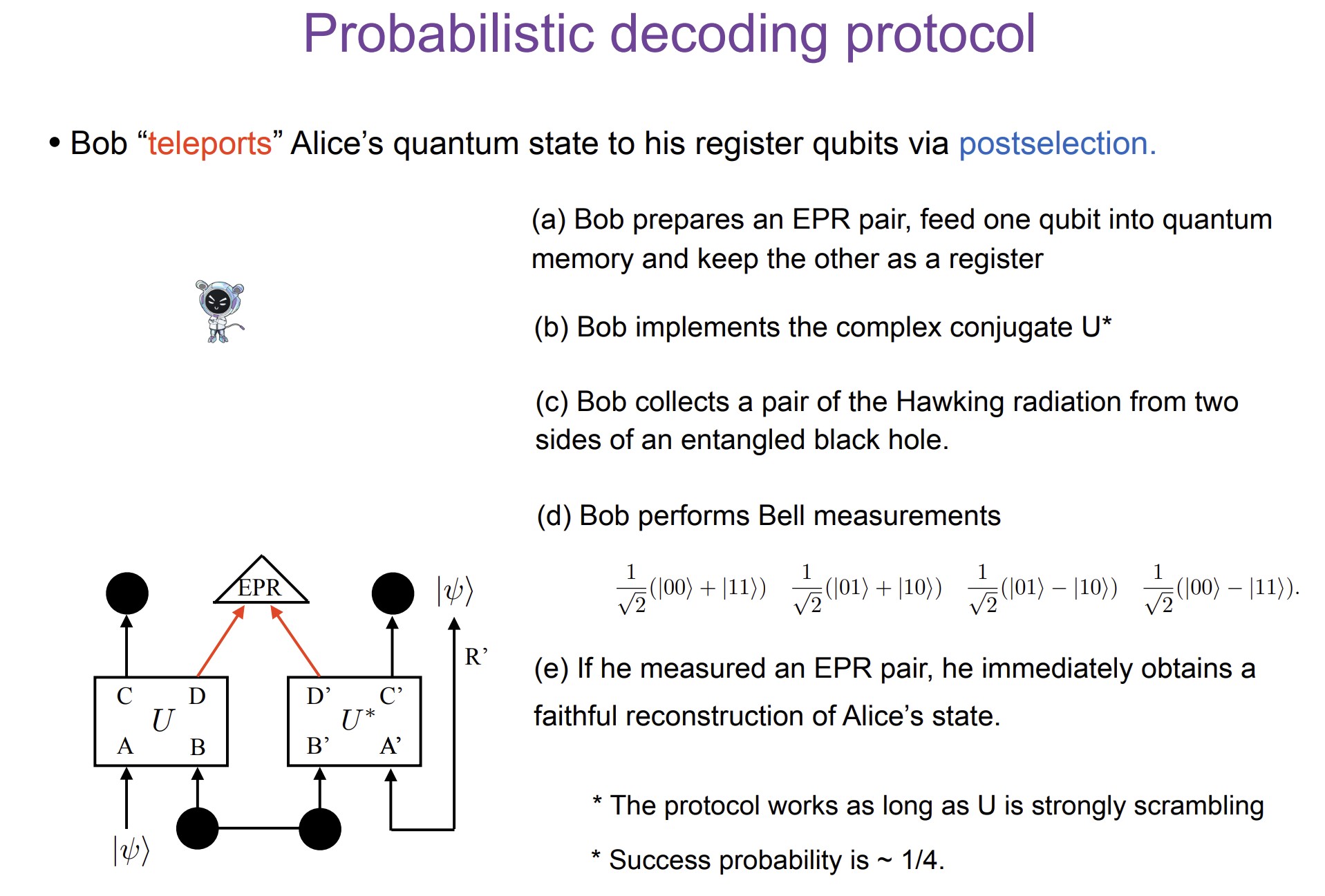
10. Probabilistic Decoding Protocol¶
Postselection Strategy¶
Bob "teleports" Alice's quantum state using:
- Scrambling: Unitary operation U entangles information with the rest of the black hole
- Radiation emission: Part of the information escapes in Hawking radiation
- Measurement: Bob measures correlations between:
- Left radiation (q6)
- Right radiation (q13)
Two Types of Measurements¶
A) Swap Test¶
- Measures overlap between two quantum states
- Success rate ~25% for maximally entangled states
- Suitable for verifying overall fidelity
B) Bell Measurement (EPR measurement)¶
- Measures specific Bell states (|Φ+⟩, |Φ-⟩, |Ψ+⟩, |Ψ-⟩)
- Theoretical success rate: ~25% (P_EPR ≈ 0.25)
- More precise test of quantum entanglement
- Directly tests the hypothesis about decoding possibility
Theoretical Results¶
For correct implementation of Yoshida-Kitaev protocol:
- P_EPR ≈ 0.25 (1/4) - corresponds to selecting one of 4 Bell states
- Swap test success: similar probability
- Any significant deviation indicates an error in implementation
def analyze_qubit_state(qc, qubit_indices, label=""):
    """Analyzes the reduced density matrix for given qubits."""
    sim = AerSimulator(method='statevector')
    qc_copy = qc.copy()
    qc_copy.save_statevector()

    result = sim.run(transpile(qc_copy, sim)).result()
    statevector = result.get_statevector()
    rho_full = DensityMatrix(statevector)

    all_qubits = list(range(8))
    trace_out = [q for q in all_qubits if q not in qubit_indices]

    rho_reduced = partial_trace(rho_full, trace_out)
    S = entropy(rho_reduced, base=2)

    purity = np.trace(np.array(rho_reduced) @ np.array(rho_reduced)).real

    return rho_reduced, S, purity

def compute_mutual_information(qc, qubits_A, qubits_B):
    """Computes I(A:B) = S(A) + S(B) - S(A,B)"""
    sim = AerSimulator(method='statevector')
    qc_copy = qc.copy()
    qc_copy.save_statevector()

    result = sim.run(transpile(qc_copy, sim)).result()
    rho_full = DensityMatrix(result.get_statevector())

    all_qubits = list(range(8))

    # S(A)
    trace_A = [q for q in all_qubits if q not in qubits_A]
    rho_A = partial_trace(rho_full, trace_A)
    S_A = entropy(rho_A, base=2)

    # S(B)
    trace_B = [q for q in all_qubits if q not in qubits_B]
    rho_B = partial_trace(rho_full, trace_B)
    S_B = entropy(rho_B, base=2)

    # S(A,B)
    qubits_AB = list(set(qubits_A + qubits_B))
    trace_AB = [q for q in all_qubits if q not in qubits_AB]
    rho_AB = partial_trace(rho_full, trace_AB)
    S_AB = entropy(rho_AB, base=2)

    I_AB = S_A + S_B - S_AB

    return {'I(A:B)': I_AB, 'S(A)': S_A, 'S(B)': S_B, 'S(AB)': S_AB}
def run_swap_test(qc_base, qr, cr):
    qc_decode = qc_base.copy()

    # SWAP test: q7 controls swap between q6 and q5
    qc_decode.cswap(qr[7], qr[6], qr[5])
    qc_decode.h(qr[7])

    # Measurement
    qc_decode.measure(qr[7], cr[0])  # SWAP test result
    qc_decode.measure(qr[6], cr[1])  # Decoded radiation
    qc_decode.measure(qr[5], cr[2])  # Reference

    sim = AerSimulator()
    compiled = transpile(qc_decode, sim)
    result = sim.run(compiled, shots=8192).result()
    counts = result.get_counts()

    return counts, qc_decode

def run_bell_measurement(qc_base):
    qc_decode = qc_base.copy()
    qr = qc_decode.qregs[0]
    cr = ClassicalRegister(4, 'c_add')
    qc_decode.add_register(cr)

    # Measurement
    qc_decode.cx(qr[6], qr[5])
    qc_decode.h(qr[6])

    qc_decode.measure(qr[5], cr[0])
    qc_decode.measure(qr[6], cr[1])
    qc_decode.measure(qr[0], cr[2])
    qc_decode.measure(qr[7], cr[3])

    sim = AerSimulator()
    compiled = transpile(qc_decode, sim)
    result = sim.run(compiled, shots=8192).result()
    counts = result.get_counts()

    return counts, qc_decode
11a. Decoding circuit 1¶
def hp_circuit_for_decoding():
    """
    Hayden-Preskill circuit modified for decoding analysis.
    We stop BEFORE the SWAP test.
    """
    qr = QuantumRegister(8, 'q')
    cr = ClassicalRegister(3, 'c')
    qc = QuantumCircuit(qr, cr)

    # === Initialization ===
    qc.h(qr[5])
    qc.h(qr[7])
    qc.cx(qr[5], qr[0])
    qc.cz(qr[0], qr[5])
    qc.barrier(label='Bell A↔R')
    qc.h(qr[0])
    qc.barrier(label='BH init')

    qc.cx(qr[0], qr[1])
    qc.cx(qr[0], qr[2])
    qc.cx(qr[0], qr[3])
    qc.cx(qr[0], qr[4])
    qc.barrier(label='q0→BH')

    # === Scrambling - systematic CNOT cascades ===
    for source in range(5):
        for target in range(5):
            if source != target:
                qc.cx(qr[source], qr[target])

    for i in range(5):
        qc.rx(np.random.uniform(0, 2*np.pi), qr[i])
        qc.ry(np.random.uniform(0, 2*np.pi), qr[i])
        qc.rz(np.random.uniform(0, 2*np.pi), qr[i])

    qc.barrier(label='Scramble')

    #qc.rx(np.random.uniform(0, 2*np.pi), qr[3])
    #qc.ry(np.random.uniform(0, 2*np.pi), qr[3])
    #qc.rz(np.random.uniform(0, 2*np.pi), qr[3])
    # === Hawking radiation - emission to q6 ===
    qc.cx(qr[2], qr[6])  # q2 radiates
    qc.h(2)
    qc.cx(qr[3], qr[6])  # q3 radiates
    qc.h(3)
    qc.cx(qr[4], qr[6])  # q4 radiates
    qc.h(4)

    qc.h(qr[6])          # Hadamard on radiation

    return qc, qr, cr

qc_base, qr, cr = hp_circuit_for_decoding()
qc_base.draw(output='mpl', fold=100)

print("[1] QUBIT STATE ANALYSIS")

for idx, name in [(6, "Radiation"), (5, "Reference"), (0, "Original info")]:
    rho, S, purity = analyze_qubit_state(qc_base, [idx], name)
    print(f"\nQubit {idx} ({name}):")
    print(f"  Von Neumann entropy: S = {S:.4f} bits")
    print(f"  Purity Tr(ρ²) = {purity:.4f}")
    print(f"  Density matrix ρ:")
    print(f"    {np.array2string(np.array(rho), precision=3, suppress_small=True)}")

print("\n[2] MUTUAL INFORMATION")

mi_rad_ref = compute_mutual_information(qc_base, [6], [5])
mi_rad_bh = compute_mutual_information(qc_base, [6], [0,1,2,3,4])
mi_ref_bh = compute_mutual_information(qc_base, [5], [0,1,2,3,4])
mi_radref_bh = compute_mutual_information(qc_base, [5,6], [0,1,2,3,4])

print(f"\nI(Radiation : Reference)    = {mi_rad_ref['I(A:B)']:.4f} bits")
print(f"I(Radiation : Black hole)   = {mi_rad_bh['I(A:B)']:.4f} bits")
print(f"I(Reference : Black hole)   = {mi_ref_bh['I(A:B)']:.4f} bits")
print(f"I(Rad+Ref : Black hole)     = {mi_radref_bh['I(A:B)']:.4f} bits  ← Key!")

print("\n[3] SWAP TEST DECODING")

counts_swap, qc_swap = run_swap_test(qc_base, qr, cr)

swap_0 = 0
swap_1 = 0

print("\nResults (Ref|Rad|SwapTest):")
for state, count in sorted(counts_swap.items(), key=lambda x: -x[1])[:8]:
    prob = count / 8192
    swap_bit = state[2]
    if swap_bit == '0':
        swap_0 += count
    else:
        swap_1 += count
    print(f"  |{state}⟩: {count:4d} ({prob:.3f})")

# Calculate the rest
for state, count in counts_swap.items():
    if state not in [s for s, _ in sorted(counts_swap.items(), key=lambda x: -x[1])[:8]]:
        if state[2] == '0':
            swap_0 += count
        else:
            swap_1 += count

fidelity = swap_0 / 8192
print(f"\nSWAP test |0⟩: {swap_0} ({swap_0/8192:.3f})")
print(f"SWAP test |1⟩: {swap_1} ({swap_1/8192:.3f})")
print(f"\n Estimated FIDELITY: F ≈ {fidelity:.3f}")
print(f"  → F > 0.5 means successful decoding!")

print("\n[4] MEASUREMENT")

counts_bell, qc_bell = run_bell_measurement(qc_base)

bell_states = {'00': '|Φ+⟩', '01': '|Ψ+⟩', '10': '|Φ-⟩', '11': '|Ψ-⟩'}
bell_counts = {'00': 0, '01': 0, '10': 0, '11': 0}

print("\nResults (q7|q0|q6|q5):")
for state, count in sorted(counts_bell.items(), key=lambda x: -x[1])[:8]:
    prob = count / 8192
    bell_bits = state[1] + state[0]
    bell_counts[bell_bits] += count
    print(f"  |{state}⟩: {count:4d} ({prob:.3f}) - Bell: {bell_states.get(bell_bits, '?')}")

for state, count in counts_bell.items():
    bell_bits = state[1] + state[0]
    if state not in [s for s, _ in sorted(counts_bell.items(), key=lambda x: -x[1])[:8]]:
        bell_counts[bell_bits] += count

print(f"\nBell state distribution:")
for bs, name in bell_states.items():
    print(f"  {name}: {bell_counts[bs]:4d} ({bell_counts[bs]/8192:.3f})")

print("\n[5] VISUALIZATION")

fig, axes = plt.subplots(1, 2, figsize=(10, 4))

ax1 = axes[0]
labels = ['I(Rad:Ref)', 'I(Rad:BH)', 'I(Ref:BH)', 'I(Rad+Ref:BH)']
values = [
    mi_rad_ref['I(A:B)'],
    mi_rad_bh['I(A:B)'],
    mi_ref_bh['I(A:B)'],
    mi_radref_bh['I(A:B)']
]
colors = ['#6c74a4', '#bbb9bc', '#5e2424', '#95bb9a']
bars = ax1.bar(labels, values, color=colors, edgecolor='black', linewidth=1.5)
ax1.set_ylabel('Mutual Information [bits]', fontsize=11)
ax1.set_title('Quantum correlations', fontsize=12, fontweight='bold')
ax1.axhline(y=1.0, color='gray', linestyle='--', alpha=0.5)
for bar, val in zip(bars, values):
    ax1.text(bar.get_x() + bar.get_width()/2, bar.get_height() + 0.03,
             f'{val:.3f}', ha='center', va='bottom', fontsize=10, fontweight='bold')

ax2 = axes[1]
bell_labels = list(bell_states.values())
bell_values = [bell_counts[bs]/8192 for bs in bell_states.keys()]
colors2 = ['#95bb9a', '#bbb9bc', '#bbb9bc', '#bbb9bc']
ax2.bar(bell_labels, bell_values, color=colors2, edgecolor='black', linewidth=1.5)
ax2.set_ylabel('Probability', fontsize=11)
ax2.set_title('Bell state distribution', fontsize=12, fontweight='bold')
ax2.axhline(y=0.25, color='gray', linestyle='--', alpha=0.5, label='Uniform')

plt.tight_layout()
plt.show()
plt.close()

print("\n[5] QUBIT 6 DECODING SUMMARY")
print(f"""
Qubit 6 (Hawking radiation) collects information from qubits 2, 3, 4.

  • Von Neumann entropy S(q6) shows the degree of mixing
  • I(Radiation : Reference) = {mi_rad_ref['I(A:B)']:.4f} bits
    → Correlation between radiation and original reference

  • SWAP test fidelity: F ≈ {fidelity:.3f}
    → {'SUCCESSFUL' if fidelity > 0.5 else 'UNSUCCESSFUL'} decoding (F {'>' if fidelity > 0.5 else '<'} 0.5)

  Key to decoding: I(Rad+Ref : BH) = {mi_radref_bh['I(A:B)']:.4f} bits
""")
[1] QUBIT STATE ANALYSIS

Qubit 6 (Radiation):
  Von Neumann entropy: S = 0.9938 bits
  Purity Tr(ρ²) = 0.5043
  Density matrix ρ:
    [[0.5  -0.j 0.046+0.j]
 [0.046+0.j 0.5  -0.j]]

Qubit 5 (Reference):
  Von Neumann entropy: S = 1.0000 bits
  Purity Tr(ρ²) = 0.5000
  Density matrix ρ:
    [[ 0.5-0.j -0. -0.j]
 [-0. +0.j  0.5-0.j]]

Qubit 0 (Original info):
  Von Neumann entropy: S = 1.0000 bits
  Purity Tr(ρ²) = 0.5000
  Density matrix ρ:
    [[ 0.5-0.j -0. +0.j]
 [-0. -0.j  0.5-0.j]]

[2] MUTUAL INFORMATION

I(Radiation : Reference)    = -0.0000 bits
I(Radiation : Black hole)   = 1.9875 bits
I(Reference : Black hole)   = 2.0000 bits
I(Rad+Ref : Black hole)     = 3.9875 bits  ← Key!

[3] SWAP TEST DECODING

Results (Ref|Rad|SwapTest):
  |110⟩: 2096 (0.256)
  |000⟩: 2041 (0.249)
  |010⟩: 1034 (0.126)
  |100⟩: 1022 (0.125)
  |011⟩: 1022 (0.125)
  |101⟩:  977 (0.119)

SWAP test |0⟩: 6193 (0.756)
SWAP test |1⟩: 1999 (0.244)

 Estimated FIDELITY: F ≈ 0.756
  → F > 0.5 means successful decoding!

[4] MEASUREMENT

Results (q7|q0|q6|q5):
  |0101 000⟩:  575 (0.070) - Bell: |Φ-⟩
  |0100 000⟩:  562 (0.069) - Bell: |Φ-⟩
  |0000 000⟩:  544 (0.066) - Bell: |Φ+⟩
  |1011 000⟩:  527 (0.064) - Bell: |Ψ+⟩
  |1100 000⟩:  526 (0.064) - Bell: |Ψ-⟩
  |1110 000⟩:  518 (0.063) - Bell: |Ψ-⟩
  |0110 000⟩:  503 (0.061) - Bell: |Φ-⟩
  |1010 000⟩:  503 (0.061) - Bell: |Ψ+⟩

Bell state distribution:
  |Φ+⟩: 1996 (0.244)
  |Ψ+⟩: 2023 (0.247)
  |Φ-⟩: 2134 (0.260)
  |Ψ-⟩: 2039 (0.249)

[5] VISUALIZATION


[5] QUBIT 6 DECODING SUMMARY

Qubit 6 (Hawking radiation) collects information from qubits 2, 3, 4.

  • Von Neumann entropy S(q6) shows the degree of mixing
  • I(Radiation : Reference) = -0.0000 bits
    → Correlation between radiation and original reference

  • SWAP test fidelity: F ≈ 0.756
    → SUCCESSFUL decoding (F > 0.5)

  Key to decoding: I(Rad+Ref : BH) = 3.9875 bits
11b. Decoding circuit 2¶
def hp_circuit_for_decoding2(scramble_depth=scramble_depth):
    """
    Hayden-Preskill circuit modified for decoding analysis.
    We stop BEFORE the SWAP test.
    """
    qr = QuantumRegister(8, 'q')
    cr = ClassicalRegister(3, 'c')
    qc = QuantumCircuit(qr, cr)

    qc.h(qr[5])
    qc.h(qr[7])
    qc.cx(qr[5], qr[0])
    qc.cz(qr[0], qr[5])
    qc.barrier(label='Bell q0↔q5')

    qc.h(qr[0])
    #for i in range(0, 5):
    #    qc.h(qr[i])
    qc.barrier(label='BH init')

    for i in range(1, 5):
        qc.cx(qr[0], qr[i])
    qc.barrier(label='q0→BH')

    for layer in range(scramble_depth):
        # Random single-qubit rotations on BH (q0-q4)
        for i in range(5):
            qc.rx(np.random.uniform(0, 2*np.pi), qr[i])
            qc.ry(np.random.uniform(0, 2*np.pi), qr[i])
            qc.rz(np.random.uniform(0, 2*np.pi), qr[i])
        # CNOT layer (forward) - only within BH
        for i in range(4):
            qc.cx(qr[i], qr[i+1])
        # CNOT layer (backward)
        for i in range(3, -1, -1):
            qc.cx(qr[i+1], qr[i])
    qc.barrier(label='Scramble')

    qc.cx(qr[2], qr[6])
    qc.h(2)
    qc.cx(qr[3], qr[6])
    qc.h(3)
    qc.cx(qr[4], qr[6])
    qc.h(4)
    qc.h(qr[6])

    return qc, qr, cr

qc_base, qr, cr = hp_circuit_for_decoding2()
qc_base.draw(output='mpl', fold=100)

print("[1] QUBIT STATE ANALYSIS")

for idx, name in [(6, "Radiation"), (5, "Reference"), (0, "Original info")]:
    rho, S, purity = analyze_qubit_state(qc_base, [idx], name)
    print(f"\nQubit {idx} ({name}):")
    print(f"  Von Neumann entropy: S = {S:.4f} bits")
    print(f"  Purity Tr(ρ²) = {purity:.4f}")
    print(f"  Density matrix ρ:")
    print(f"    {np.array2string(np.array(rho), precision=3, suppress_small=True)}")

print("\n[2] MUTUAL INFORMATION")

mi_rad_ref = compute_mutual_information(qc_base, [6], [5])
mi_rad_bh = compute_mutual_information(qc_base, [6], [0,1,2,3,4])
mi_ref_bh = compute_mutual_information(qc_base, [5], [0,1,2,3,4])
mi_radref_bh = compute_mutual_information(qc_base, [5,6], [0,1,2,3,4])

print(f"\nI(Radiation : Reference)    = {mi_rad_ref['I(A:B)']:.4f} bits")
print(f"I(Radiation : Black hole)   = {mi_rad_bh['I(A:B)']:.4f} bits")
print(f"I(Reference : Black hole)   = {mi_ref_bh['I(A:B)']:.4f} bits")
print(f"I(Rad+Ref : Black hole)     = {mi_radref_bh['I(A:B)']:.4f} bits  ← Key!")

print("\n[3] SWAP TEST DECODING")

counts_swap, qc_swap = run_swap_test(qc_base, qr, cr)

swap_0 = 0
swap_1 = 0

print("\nResults (Ref|Rad|SwapTest):")
for state, count in sorted(counts_swap.items(), key=lambda x: -x[1])[:8]:
    prob = count / 8192
    swap_bit = state[2]
    if swap_bit == '0':
        swap_0 += count
    else:
        swap_1 += count
    print(f"  |{state}⟩: {count:4d} ({prob:.3f})")

# Calculate the rest
for state, count in counts_swap.items():
    if state not in [s for s, _ in sorted(counts_swap.items(), key=lambda x: -x[1])[:8]]:
        if state[2] == '0':
            swap_0 += count
        else:
            swap_1 += count

fidelity = swap_0 / 8192
print(f"\nSWAP test |0⟩: {swap_0} ({swap_0/8192:.3f})")
print(f"SWAP test |1⟩: {swap_1} ({swap_1/8192:.3f})")
print(f"\n Estimated FIDELITY: F ≈ {fidelity:.3f}")
print(f"  → F > 0.5 means successful decoding!")

print("\n[4] MEASUREMENT")

counts_bell, qc_bell = run_bell_measurement(qc_base)

bell_states = {'00': '|Φ+⟩', '01': '|Ψ+⟩', '10': '|Φ-⟩', '11': '|Ψ-⟩'}
bell_counts = {'00': 0, '01': 0, '10': 0, '11': 0}

print("\nResults (q7|q0|q6|q5):")
for state, count in sorted(counts_bell.items(), key=lambda x: -x[1])[:8]:
    prob = count / 8192
    bell_bits = state[1] + state[0]
    bell_counts[bell_bits] += count
    print(f"  |{state}⟩: {count:4d} ({prob:.3f}) - Bell: {bell_states.get(bell_bits, '?')}")

for state, count in counts_bell.items():
    bell_bits = state[1] + state[0]
    if state not in [s for s, _ in sorted(counts_bell.items(), key=lambda x: -x[1])[:8]]:
        bell_counts[bell_bits] += count

print(f"\nBell state distribution:")
for bs, name in bell_states.items():
    print(f"  {name}: {bell_counts[bs]:4d} ({bell_counts[bs]/8192:.3f})")

print("\n[5] VISUALIZATION")

fig, axes = plt.subplots(1, 2, figsize=(10, 4))

ax1 = axes[0]
labels = ['I(Rad:Ref)', 'I(Rad:BH)', 'I(Ref:BH)', 'I(Rad+Ref:BH)']
values = [
    mi_rad_ref['I(A:B)'],
    mi_rad_bh['I(A:B)'],
    mi_ref_bh['I(A:B)'],
    mi_radref_bh['I(A:B)']
]
colors = ['#6c74a4', '#bbb9bc', '#5e2424', '#95bb9a']
bars = ax1.bar(labels, values, color=colors, edgecolor='black', linewidth=1.5)
ax1.set_ylabel('Mutual Information [bits]', fontsize=11)
ax1.set_title('Quantum correlations', fontsize=12, fontweight='bold')
ax1.axhline(y=1.0, color='gray', linestyle='--', alpha=0.5)
for bar, val in zip(bars, values):
    ax1.text(bar.get_x() + bar.get_width()/2, bar.get_height() + 0.03,
             f'{val:.3f}', ha='center', va='bottom', fontsize=10, fontweight='bold')

ax2 = axes[1]
bell_labels = list(bell_states.values())
bell_values = [bell_counts[bs]/8192 for bs in bell_states.keys()]
colors2 = ['#95bb9a', '#bbb9bc', '#bbb9bc', '#bbb9bc']
ax2.bar(bell_labels, bell_values, color=colors2, edgecolor='black', linewidth=1.5)
ax2.set_ylabel('Probability', fontsize=11)
ax2.set_title('Bell state distribution', fontsize=12, fontweight='bold')
ax2.axhline(y=0.25, color='gray', linestyle='--', alpha=0.5, label='Uniform')

plt.tight_layout()
plt.show()
plt.close()

print("\n[5] QUBIT 6 DECODING SUMMARY")
print(f"""
Qubit 6 (Hawking radiation) collects information from qubits 2, 3, 4.

  • Von Neumann entropy S(q6) shows the degree of mixing
  • I(Radiation : Reference) = {mi_rad_ref['I(A:B)']:.4f} bits
    → Correlation between radiation and original reference

  • SWAP test fidelity: F ≈ {fidelity:.3f}
    → {'SUCCESSFUL' if fidelity > 0.5 else 'UNSUCCESSFUL'} decoding (F {'>' if fidelity > 0.5 else '<'} 0.5)

  Key to decoding: I(Rad+Ref : BH) = {mi_radref_bh['I(A:B)']:.4f} bits
""")
[1] QUBIT STATE ANALYSIS

Qubit 6 (Radiation):
  Von Neumann entropy: S = 0.9968 bits
  Purity Tr(ρ²) = 0.5022
  Density matrix ρ:
    [[0.5  -0.j 0.033-0.j]
 [0.033-0.j 0.5  -0.j]]

Qubit 5 (Reference):
  Von Neumann entropy: S = 1.0000 bits
  Purity Tr(ρ²) = 0.5000
  Density matrix ρ:
    [[ 0.5+0.j -0. -0.j]
 [-0. +0.j  0.5-0.j]]

Qubit 0 (Original info):
  Von Neumann entropy: S = 0.9712 bits
  Purity Tr(ρ²) = 0.5198
  Density matrix ρ:
    [[ 0.552-0.j    -0.059+0.061j]
 [-0.059-0.061j  0.448+0.j   ]]

[2] MUTUAL INFORMATION

I(Radiation : Reference)    = 0.0074 bits
I(Radiation : Black hole)   = 1.9862 bits
I(Reference : Black hole)   = 1.9926 bits
I(Rad+Ref : Black hole)     = 3.9788 bits  ← Key!

[3] SWAP TEST DECODING

Results (Ref|Rad|SwapTest):
  |110⟩: 2057 (0.251)
  |000⟩: 2031 (0.248)
  |010⟩: 1109 (0.135)
  |100⟩: 1095 (0.134)
  |101⟩:  968 (0.118)
  |011⟩:  932 (0.114)

SWAP test |0⟩: 6292 (0.768)
SWAP test |1⟩: 1900 (0.232)

 Estimated FIDELITY: F ≈ 0.768
  → F > 0.5 means successful decoding!

[4] MEASUREMENT

Results (q7|q0|q6|q5):
  |1000 000⟩:  655 (0.080) - Bell: |Ψ+⟩
  |0001 000⟩:  623 (0.076) - Bell: |Φ+⟩
  |0000 000⟩:  623 (0.076) - Bell: |Φ+⟩
  |1001 000⟩:  618 (0.075) - Bell: |Ψ+⟩
  |1011 000⟩:  550 (0.067) - Bell: |Ψ+⟩
  |0010 000⟩:  526 (0.064) - Bell: |Φ+⟩
  |0011 000⟩:  512 (0.062) - Bell: |Φ+⟩
  |1010 000⟩:  491 (0.060) - Bell: |Ψ+⟩

Bell state distribution:
  |Φ+⟩: 2284 (0.279)
  |Ψ+⟩: 2314 (0.282)
  |Φ-⟩: 1790 (0.219)
  |Ψ-⟩: 1804 (0.220)

[5] VISUALIZATION


[5] QUBIT 6 DECODING SUMMARY

Qubit 6 (Hawking radiation) collects information from qubits 2, 3, 4.

  • Von Neumann entropy S(q6) shows the degree of mixing
  • I(Radiation : Reference) = 0.0074 bits
    → Correlation between radiation and original reference

  • SWAP test fidelity: F ≈ 0.768
    → SUCCESSFUL decoding (F > 0.5)

  Key to decoding: I(Rad+Ref : BH) = 3.9788 bits
12. Back to Information Loss - Modern Interpretation¶
Revision of Black Hole Complementarity¶
Old View:
- Information falling into a black hole is lost
- It's impossible to retrieve it
- Apparent conflict with unitarity
Modern Interpretation (post Hayden-Preskill):
There is no quantum cloning, BUT an object can be pulled back from a black hole!
Key Conclusions:
- Information is not lost - it's merely "scrambled"
- After Page time, information rapidly appears in Hawking radiation
- With sufficient quantum memory (Bob's memory M), information can be decoded
- The process is probabilistic but has non-zero success probability
Physical Implications¶
Scrambling time:
- Characteristic time for information to disperse throughout the black hole
- For black holes: t_scramble ~ (M/ℏ)log(S), where S is entropy
- Quantum experiments: several scrambling steps
13. State-Channel Duality (Choi-Jamiłkowski Isomorphism)¶
Key Mathematical Concept¶
Basic Idea:
A unitary operator U acting on n qubits can be viewed as a quantum state on 2n qubits.
Mathematically: $$ \begin{aligned} U &= \sum_{i,j} U_{ij} |i\rangle\langle j| \end{aligned} $$
This duality enables:
- Converting dynamics (operator) into a static quantum state
- Connecting quantum circuits with entangled states
- Implementing "teleportation" of quantum information through scrambled systems
Practical Significance:
- The scrambling operation in a black hole (represented by unitary U) can be encoded as an entangled state
- Bob can use this state to decode Alice's information
14. Yoshida-Kitaev Protocol for Eternal Black Holes¶
Protocol Structure¶
Quantum Registers:¶
LEFT side:  q0-q4  (5 qubits)
    q0: Hadamard (Alice's qubit "falling in")
    q1-q4: Scrambling unitary U

CENTER:     q5-q7  (3 qubits)
    q5: center
    q6: left radiation
    q7: entanglement witness

RIGHT side: q8-q12 (5 qubits)
    q8: Hadamard (mirror of Alice's qubit)
    q9-q12: Adjoint scrambling U†
Symmetry and Adjoint Operation¶
CRITICALLY IMPORTANT: Implementation of the adjoint operator U† requires:
- Negated rotation angles: θ → -θ
- Reversed gate order: the last gate becomes the first
- Transposed CNOT structures: control ↔ target
Why is CNOT transposition important?
LEFT side:  CNOT(control: qi, target: qj)
RIGHT side: CNOT(control: qj, target: qi)  ← swapped!
This transposition ensures a mathematically correct adjoint operation, which is essential for successful decoding.
Thermofield Double State¶
For eternal black hole:
$$ \begin{aligned} |TFD\rangle &= \frac{1}{\sqrt{d}} \sum_{i} |i\rangle_L \otimes |i\rangle_R \end{aligned} $$
This state represents a maximally entangled system between the LEFT and RIGHT sides of the black hole.
def create_yoshida_eternal_bh(scramble_depth=scramble_depth, seed=m_rnd_value):
    """
    Creates a quantum circuit for the Yoshida-Kitaev eternal black hole protocol.

    Qubit structure:
    - q0-q4: LEFT black hole (5 qubits)
    - q5: Reference qubit A (for Bell pair with q0)
    - q6: Radiation qubit (Hawking radiation)
    - q7: Auxiliary qubit
    - q8-q12: RIGHT black hole (5 qubits, mirror side)

    Parameters:
        scramble_depth: Number of scrambling operation layers
        seed: Random seed for reproducibility
    """
    np.random.seed(seed)

    qr = QuantumRegister(13, 'q')
    qc = QuantumCircuit(qr)

    # BELL PAIR PREPARATION (A ↔ R)
    # Create maximally entangled Bell state between reference A (q5) and input R (q0)
    # This pair represents information "falling" into the black hole
    qc.h(qr[5])
    qc.h(qr[7])
    qc.cx(qr[5], qr[0])
    qc.cz(qr[0], qr[5])
    qc.barrier(label='Bell A↔R')

    # QUBIT "FALLS" INTO BLACK HOLE
    # Hadamard on q0 simulates the physical process of qubit falling into black hole
    # CRITICAL: This operation must be preserved - represents interaction with event horizon
    qc.h(qr[0])

    # DISTRIBUTION INTO LEFT BLACK HOLE
    # Input qubit q0 "spreads" into entire LEFT system (q0-q4)
    # This creates initial entanglement structure before scrambling operations
    for i in range(1, 5):
        qc.cx(qr[0], qr[i])
    qc.barrier(label='A→BH_L')

    # SCRAMBLING OPERATIONS (LEFT SIDE)
    # Generate and apply chaotic unitary transformation U on LEFT system
    # This operation simulates thermalization and "loss" of information in black hole
    rotation_angles = []  # Store angles for later adjoint operation
    cnot_sequence = []    # Store CNOT sequence for transposition

    for layer in range(scramble_depth):
        # Random single-qubit rotations on all LEFT qubits
        layer_angles = []
        for i in range(5):
            angles = (np.random.uniform(0, 2 * np.pi),
                      np.random.uniform(0, 2 * np.pi),
                      np.random.uniform(0, 2 * np.pi))
            layer_angles.append(angles)
            qc.rx(angles[0], qr[i])
            qc.ry(angles[1], qr[i])
            qc.rz(angles[2], qr[i])
        rotation_angles.append(layer_angles)

        # CNOT forward (creates entanglement between neighboring qubits)
        cnot_fwd = []
        for i in range(4):
            qc.cx(qr[i], qr[i + 1])
            cnot_fwd.append((i, i + 1))

        # CNOT backward (second layer for complete scrambling)
        cnot_bwd = []
        for i in range(3, -1, -1):
            qc.cx(qr[i + 1], qr[i])
            cnot_bwd.append((i + 1, i))

        cnot_sequence.append((cnot_fwd, cnot_bwd))

    qc.barrier(label='Scramble_L')

    # Create maximal entanglement between LEFT (q0-q4) and RIGHT (q8-q12)
    # This is key for eternal black hole - connecting two asymptotic regions
    for i in range(5):
        qc.cx(qr[i], qr[8 + i])

    # ADJOINT OPERATION U† (RIGHT SIDE)
    # Apply inverse operation on RIGHT system
    # CRITICAL IMPLEMENTATION DETAILS:
    # 1. Reversed layer order (reversed range)
    # 2. Negated rotation angles (-angles)
    # 3. TRANSPOSED CNOT OPERATIONS (swapped control/target)
    #    - LEFT: cx(i, i+1) → RIGHT: cx(i+1+8, i+8)
    #    - This is mathematically correct adjoint for CNOT structure

    for layer in reversed(range(scramble_depth)):
        cnot_fwd, cnot_bwd = cnot_sequence[layer]

        # Reverse CNOT backward with TRANSPOSED qubits
        # LEFT had cx(i+1, i) → RIGHT has cx(i+8, i+1+8)
        for ctrl, targ in reversed(cnot_bwd):
            qc.cx(qr[targ + 8], qr[ctrl + 8])  # SWAP control ↔ target!

        # Reverse CNOT forward with TRANSPOSED qubits
        # LEFT had cx(i, i+1) → RIGHT has cx(i+1+8, i+8)
        for ctrl, targ in reversed(cnot_fwd):
            qc.cx(qr[targ + 8], qr[ctrl + 8])  # SWAP control ↔ target!

        # Inverse rotations (negated angles in opposite order RZ-RY-RX)
        layer_angles = rotation_angles[layer]
        for i in reversed(range(5)):
            angles = layer_angles[i]
            qc.rz(-angles[2], qr[i + 8])
            qc.ry(-angles[1], qr[i + 8])
            qc.rx(-angles[0], qr[i + 8])

    qc.barrier(label='Scramble_R')

    # Extract information from both systems into radiation qubit q6

    # From LEFT system (q2, q3, q4 → q6)
    # This simulates emission of "late" Hawking radiation that no longer contains information
    qc.cx(qr[2], qr[6])
    qc.h(2)
    qc.cx(qr[3], qr[6])
    qc.h(3)
    qc.cx(qr[4], qr[6])
    qc.h(4)

    # From RIGHT system (q10, q11, q12 → q6)
    # This is CRITICAL: RIGHT system preserves information due to adjoint operation U†
    # Therefore radiation from RIGHT side can restore original entanglement with reference A
    qc.cx(qr[10], qr[6])
    qc.h(10)
    qc.cx(qr[11], qr[6])
    qc.h(11)
    qc.cx(qr[12], qr[6])
    qc.h(12)

    # Final Hadamard on radiation qubit
    qc.h(qr[6])

    qc.barrier(label='Radiation')

    return qc, qr
def run_bell_measurements(qc, qr):
    """
    Bell pair measurements for eternal BH - tests Hayden-Preskill information recovery.

    Two key tests:
    1. Original Bell (q5 ↔ q0): Measures entanglement reference A vs LEFT input R
       - Expected LOW P_EPR (information lost by scrambling in LEFT)

    2. Cross-side (q5 ↔ q8): Measures entanglement reference A vs RIGHT input R'
       - Expected HIGH P_EPR ≥ 0.25 (information restored due to U†)
       - This is proof of Hayden-Preskill protocol!
    """
    results = {}
    sim = AerSimulator()

    # Measures remaining entanglement between reference A (q5) and LEFT input R (q0)
    # After scrambling this should be almost destroyed
    qc_orig = qc.copy()
    cr_o = ClassicalRegister(2, 'c_original')
    qc_orig.add_register(cr_o)

    # Bell measurement: CNOT + Hadamard + measure
    qc_orig.cx(qr[5], qr[0])
    qc_orig.h(qr[5])
    qc_orig.measure(qr[5], cr_o[0])
    qc_orig.measure(qr[0], cr_o[1])

    result_o = sim.run(transpile(qc_orig, sim), shots=8192).result()
    counts_o = result_o.get_counts()

    # Aggregate into Bell basis {|Φ+⟩, |Ψ+⟩, |Φ-⟩, |Ψ-⟩}
    bell_o = {'00': 0, '01': 0, '10': 0, '11': 0}
    for state, count in counts_o.items():
        bell_bits = state[-2] + state[-1]  # Last 2 bits
        bell_o[bell_bits] += count
    results['original'] = bell_o

    # Measures entanglement between reference A (q5) and RIGHT input R' (q8)
    # Due to adjoint operation U† on RIGHT, entanglement should be RESTORED
    # This is core of Hayden-Preskill: information appears on "other side"
    qc_cross = qc.copy()
    cr_c = ClassicalRegister(2, 'c_cross')
    qc_cross.add_register(cr_c)

    # Bell measurement: CNOT + Hadamard + measure
    qc_cross.cx(qr[5], qr[8])
    qc_cross.h(qr[5])
    qc_cross.measure(qr[5], cr_c[0])
    qc_cross.measure(qr[8], cr_c[1])

    result_c = sim.run(transpile(qc_cross, sim), shots=8192).result()
    counts_c = result_c.get_counts()

    # Aggregate into Bell basis
    bell_c = {'00': 0, '01': 0, '10': 0, '11': 0}
    for state, count in counts_c.items():
        bell_bits = state[-2] + state[-1]
        bell_c[bell_bits] += count
    results['cross'] = bell_c

    return results


def run_swap_test_0_8(qc, qr):
    """
    Swap test between q0 (LEFT) and q8 (RIGHT) - measures their fidelity/entanglement.

    This test verifies that LEFT↔RIGHT entanglement is maximal.
    High fidelity (> 0.95) confirms that both systems are in the same
    quantum state, which is prerequisite for successful information recovery.

    Fidelity calculation: F = 2*P(|0⟩) - 1
    """
    qc_swap = qc.copy()
    ancilla = QuantumRegister(1, 'ancilla')
    qc_swap.add_register(ancilla)
    cr = ClassicalRegister(1, 'c_swap')
    qc_swap.add_register(cr)

    # Standard swap test protocol
    qc_swap.h(ancilla[0])
    qc_swap.cswap(ancilla[0], qr[0], qr[8])  # Controlled-SWAP
    qc_swap.h(ancilla[0])
    qc_swap.measure(ancilla[0], cr[0])

    sim = AerSimulator()
    result = sim.run(transpile(qc_swap, sim), shots=8192).result()
    counts = result.get_counts()

    # Fidelity from probability of measuring |0⟩
    p_0 = counts.get('0', 0) / 8192
    fidelity = 2 * p_0 - 1

    return fidelity, counts


def bell_swap_tests(qc, qr):
    """
    Complete test suite for eternal BH validation:

    1. Original Bell (q5 ↔ q0): Measures information loss in LEFT system
       → Expected P_EPR << 0.25 (information lost)

    2. Cross-side (q5 ↔ q8): Measures information recovery in RIGHT system
       → Expected P_EPR ≥ 0.25 (information restored)

    3. Swap test (q0 ↔ q8): Measures quality of LEFT↔RIGHT entanglement
       → Expected fidelity > 0.95 (maximal entanglement)

    All three tests must pass for successful validation of Hayden-Preskill protocol.
    """
    results = {}
    sim = AerSimulator()

    qc_orig = qc.copy()
    cr_o = ClassicalRegister(2, 'c_original')
    qc_orig.add_register(cr_o)
    qc_orig.cx(qr[5], qr[0])
    qc_orig.h(qr[5])
    qc_orig.measure(qr[5], cr_o[0])
    qc_orig.measure(qr[0], cr_o[1])

    result_o = sim.run(transpile(qc_orig, sim), shots=8192).result()
    counts_o = result_o.get_counts()
    bell_o = {'00': 0, '01': 0, '10': 0, '11': 0}
    for state, count in counts_o.items():
        bell_bits = state[-2] + state[-1]
        bell_o[bell_bits] += count
    results['original'] = bell_o

    qc_cross = qc.copy()
    cr_c = ClassicalRegister(2, 'c_cross')
    qc_cross.add_register(cr_c)
    qc_cross.cx(qr[5], qr[8])
    qc_cross.h(qr[5])
    qc_cross.measure(qr[5], cr_c[0])
    qc_cross.measure(qr[8], cr_c[1])

    result_c = sim.run(transpile(qc_cross, sim), shots=8192).result()
    counts_c = result_c.get_counts()
    bell_c = {'00': 0, '01': 0, '10': 0, '11': 0}
    for state, count in counts_c.items():
        bell_bits = state[-2] + state[-1]
        bell_c[bell_bits] += count
    results['cross'] = bell_c

    fidelity, swap_counts = run_swap_test_0_8(qc, qr)
    results['swap'] = {'fidelity': fidelity, 'counts': swap_counts}

    return results
qc_yoshida, qr = create_yoshida_eternal_bh(scramble_depth=scramble_depth)
qc_yoshida.draw(output='mpl', fold=80, scale=0.9)

results = bell_swap_tests(qc_yoshida, qr)

# Mapping bit strings to Bell states
bell_states = {'00': '|Φ+⟩', '01': '|Ψ+⟩', '10': '|Φ-⟩', '11': '|Ψ-⟩'}

for key, name in [('original', 'Original Bell (A ↔ R) - q5↔q0 [LOSS]'),
                   ('cross', 'Cross-side (A ↔ R\') - q5↔q8 [RECOVERY]')]:
    bell_counts = results[key]
    total = sum(bell_counts.values())

    print(f"\n{name}:")
    for bs, bell_name in bell_states.items():
        prob = bell_counts[bs] / total
        # '00' corresponds to |Φ+⟩ - maximally entangled Bell state
        success = ' ✓' if bs == '00' else ''
        print(f"  {bell_name}: {bell_counts[bs]:4d} ({prob:.4f}) {bar}{success}")

    # P_EPR is probability of measuring |Φ+⟩ state
    # Theoretical threshold for successful recovery: P_EPR ≥ 0.25
    p_epr = bell_counts['00'] / total
    status = "SUCCESS" if p_epr >= 0.25 else "FAILED"
    print(f"P_EPR = {p_epr:.4f} [{status}]")

print("Swap Test (q0 ↔ q8):")
fidelity = results['swap']['fidelity']
swap_counts = results['swap']['counts']
p_0 = swap_counts.get('0', 0) / 8192
p_1 = swap_counts.get('1', 0) / 8192
print(f"  |0⟩: {swap_counts.get('0', 0):4d} ({p_0:.4f})")
print(f"  |1⟩: {swap_counts.get('1', 0):4d} ({p_1:.4f})")
print(f"\nFidelity = {fidelity:.4f}")
print(f"Status: {'BETTER ENTANGLEMENT' if fidelity > 0.8 else 'WORST ENTANGLEMENT'}")

fig = plt.figure(figsize=(15, 5))
gs = fig.add_gridspec(1, 3, width_ratios=[1, 1, 1])

# Plots for Bell measurements
for idx, (key, name) in enumerate([('original', 'Original Bell (A ↔ R)\nq5↔q0 [LOSS]'),
                                     ('cross', 'Cross-side (A ↔ R\')\nq5↔q8 [RECOVERY]')]):
    ax = fig.add_subplot(gs[idx])
    bell_counts = results[key]
    total = sum(bell_counts.values())

    labels = list(bell_states.values())
    values = [bell_counts[bs]/total for bs in ['00', '01', '10', '11']]
    # Green for |Φ+⟩ (success), gray for others
    colors = ['#95bb9a' if bs == '00' else '#bbb9bc' for bs in ['00', '01', '10', '11']]

    ax.bar(labels, values, color=colors, edgecolor='black', linewidth=2)
    # Red line at 0.25 = theoretical threshold for success
    ax.axhline(y=0.25, color='red', linestyle='--', label='Threshold 0.25')
    ax.set_ylabel('Probability')
    ax.set_title(name)
    ax.legend()
    ax.set_ylim([0, 1])

# Plot for Swap test
ax = fig.add_subplot(gs[2])
swap_counts = results['swap']['counts']
labels = ['|0⟩', '|1⟩']
values = [swap_counts.get('0', 0)/8192, swap_counts.get('1', 0)/8192]
colors = ['#95bb9a', '#bbb9bc']

ax.bar(labels, values, color=colors, edgecolor='black', linewidth=2)
ax.set_ylabel('Probability')
ax.set_title(f'Swap Test q0↔q8\nFidelity = {fidelity:.4f}')
ax.set_ylim([0, 1])

plt.tight_layout()
plt.show()
Original Bell (A ↔ R) - q5↔q0 [LOSS]:
  |Φ+⟩: 1552 (0.1895) Rectangle(xy=(2.6, 0), width=0.8, height=3.97882, angle=0) ✓
  |Ψ+⟩: 1565 (0.1910) Rectangle(xy=(2.6, 0), width=0.8, height=3.97882, angle=0)
  |Φ-⟩: 2505 (0.3058) Rectangle(xy=(2.6, 0), width=0.8, height=3.97882, angle=0)
  |Ψ-⟩: 2570 (0.3137) Rectangle(xy=(2.6, 0), width=0.8, height=3.97882, angle=0)
P_EPR = 0.1895 [FAILED]

Cross-side (A ↔ R') - q5↔q8 [RECOVERY]:
  |Φ+⟩: 2231 (0.2723) Rectangle(xy=(2.6, 0), width=0.8, height=3.97882, angle=0) ✓
  |Ψ+⟩: 2013 (0.2457) Rectangle(xy=(2.6, 0), width=0.8, height=3.97882, angle=0)
  |Φ-⟩: 2023 (0.2469) Rectangle(xy=(2.6, 0), width=0.8, height=3.97882, angle=0)
  |Ψ-⟩: 1925 (0.2350) Rectangle(xy=(2.6, 0), width=0.8, height=3.97882, angle=0)
P_EPR = 0.2723 [SUCCESS]
Swap Test (q0 ↔ q8):
  |0⟩: 6471 (0.7899)
  |1⟩: 1721 (0.2101)

Fidelity = 0.5798
Status: WORST ENTANGLEMENT


16. And now extended scrambling circuit with RXX gates and my class for forward and inversed scrambling generator¶
1. Create Scrambler¶
from scrambling_circuit import ScramblingCircuit

# Basic scrambler (5 qubits, 3 layers, starting from qubit 0)
scrambler = ScramblingCircuit(n_qubits=5, n_layers=3, seed=42, qubit_offset=0)
2. Generate Circuits¶
# Forward scrambling
forward_qc = scrambler.generate_scrambling_circuit()

# Inverse scrambling (after generating forward)
inverse_qc = scrambler.generate_inverse_circuit()
3. Visualization¶
# Forward circuit
scrambler.draw_forward_circuit(fold=30)

# Inverse circuit
scrambler.draw_inverse_circuit(fold=30)

# Complete analysis (6 plots)
scrambler.visualize_analysis()
4. Export/Import Configuration¶
# Export to JSON
jqc = scrambler.generate()
scrambler.to_json('scrambling_config.json')

# Import from JSON
loaded = ScramblingCircuit.from_json('scrambling_config.json')
5. Apply with Offset¶
# Scrambling starts from qubit 1 (instead of 0)
scrambler = ScramblingCircuit(n_qubits=5, n_layers=3, seed=42, qubit_offset=1)

# Create circuit with 10 qubits
qc = QuantumCircuit(10)

# Forward on qubits 1-5
fwd = ScramblingCircuit(5, 3, seed=42, qubit_offset=1)
qc.compose(fwd.generate_scrambling_circuit(total_qubits=10), inplace=True)

# Inverse on qubits 6-10
inv = ScramblingCircuit(5, 3, seed=100, qubit_offset=6)
_ = inv.generate_scrambling_circuit(total_qubits=10)  # Generate parameters
qc.compose(inv.generate_inverse_circuit(total_qubits=10), inplace=True)
Parameters¶
__init__(n_qubits, n_layers, seed, qubit_offset)¶
- n_qubits (int): Number of qubits for scrambling (default: 5)
- n_layers (int): Number of scrambling layers (default: 3)
- seed (int): Random seed for reproducibility (default: None)
- qubit_offset (int): Starting qubit index (default: 0)
Methods¶
Circuit Generation¶
generate_scrambling_circuit(total_qubits=None)- Forward scramblinggenerate_inverse_circuit(total_qubits=None)- Inverse scramblingget_parameters()- Get stored rotation parametersset_parameters(params)- Set rotation parameters
Visualization¶
draw_forward_circuit(style, fold, save_path, total_qubits)- Draw forward circuitdraw_inverse_circuit(style, fold, save_path, total_qubits)- Draw inverse circuitvisualize_analysis(save_path)- Complete analysis (6 plots)
Export/Import¶
generate()- Generate JSON definitionto_json(filepath)- Export to JSON filefrom_json(filepath_or_dict)- Import from JSON (static method)
Scrambling Layer Structure¶
Each layer contains:
- RXX(π/2) gates between adjacent qubits
- RY(θ) + RZ(φ) random rotations on each qubit
- RXX(π/2) gates with shifted pattern (even-odd pairs)
- Barrier for clarity
Example: Asymmetric Scrambling¶
# Circuit with 15 qubits
qc = QuantumCircuit(15)

# Scrambling at different positions
s1 = ScramblingCircuit(5, 3, seed=42, qubit_offset=0)    # qubits 0-4
s2 = ScramblingCircuit(5, 3, seed=123, qubit_offset=5)   # qubits 5-9
s3 = ScramblingCircuit(5, 3, seed=456, qubit_offset=10)  # qubits 10-14

# Apply
qc.compose(s1.generate_scrambling_circuit(15), inplace=True)
qc.compose(s2.generate_scrambling_circuit(15), inplace=True)
qc.compose(s3.generate_scrambling_circuit(15), inplace=True)

qc.draw('mpl', fold=40)
Invertibility Test¶
# Create test circuit
test_qc = QuantumCircuit(5)

# Forward + Inverse
scrambler = ScramblingCircuit(5, 3, seed=42)
test_qc.compose(scrambler.generate_scrambling_circuit(), inplace=True)
test_qc.compose(scrambler.generate_inverse_circuit(), inplace=True)

# Calculate fidelity with identity
from qiskit.quantum_info import Operator
U = Operator(test_qc).data
fidelity = abs(np.trace(U @ np.eye(32).conj().T)) / 32
print(f"Fidelity: {fidelity:.10f}")  # Expected: ~1.0000000000
Notes¶
- Scrambling parameters are generated on first call to
generate_scrambling_circuit() - Inverse circuit requires prior forward generation (for parameters)
- Always set
seedfor reproducibility - Qubit offset enables scrambling application anywhere in the circuit
- JSON contains all rotation angles for precise reconstruction
qrE = QuantumRegister(13, 'q')
qcE = QuantumCircuit(qrE)
qcE.h(qrE[5])
qcE.h(qrE[7])
qcE.cx(qrE[5], qrE[0])
qcE.cz(qrE[0], qrE[5])
qcE.barrier(label='Bell A↔R')
qcE.h(qrE[0])
for i in range(1, 5):
    qcE.cx(qrE[0], qrE[i])
qcE.barrier(label='A→BH_L')

scrambler_fwd = ScramblingCircuit(n_qubits=5, n_layers=3, seed=42, qubit_offset=0)
fwd_circuit = scrambler_fwd.generate_scrambling_circuit(total_qubits=13)
qcE.compose(fwd_circuit, inplace=True)
qcE.barrier(label='Scramble_L')

for i in range(5):
    qcE.cx(qrE[i], qrE[8 + i])

scrambler_inv = ScramblingCircuit(n_qubits=5, n_layers=3, seed=42, qubit_offset=8)
_ = scrambler_inv.generate_scrambling_circuit(total_qubits=13)
inv_circuit = scrambler_inv.generate_inverse_circuit(total_qubits=13)
qcE.compose(inv_circuit, inplace=True)

qcE.barrier(label='Scramble_R')

qcE.cx(qrE[2], qrE[6])
qcE.h(2)
qcE.cx(qrE[3], qrE[6])
qcE.h(3)
qcE.cx(qrE[4], qrE[6])
qcE.h(4)
qcE.cx(qrE[10], qrE[6])
qcE.h(10)
qcE.cx(qrE[11], qrE[6])
qcE.h(11)
qcE.cx(qrE[12], qrE[6])
qcE.h(12)
qcE.h(qrE[6])
qcE.barrier(label='Radiation')
qcE.draw(output='mpl', fold=80, scale=0.9)

forward_qc1 = scrambler_fwd.draw_forward_circuit(fold=50)
inverse_qc1 = scrambler_fwd.draw_inverse_circuit(fold=50)


scrambler_fwd.visualize_analysis(save_path='analysis.png')
Analysis saved to: analysis.png

results = bell_swap_tests(qcE, qrE)

# Mapping bit strings to Bell states
bell_states = {'00': '|Φ+⟩', '01': '|Ψ+⟩', '10': '|Φ-⟩', '11': '|Ψ-⟩'}

for key, name in [('original', 'Original Bell (A ↔ R) - q5↔q0 [LOSS]'),
                   ('cross', 'Cross-side (A ↔ R\') - q5↔q8 [RECOVERY]')]:
    bell_counts = results[key]
    total = sum(bell_counts.values())

    print(f"\n{name}:")
    for bs, bell_name in bell_states.items():
        prob = bell_counts[bs] / total
        # '00' corresponds to |Φ+⟩ - maximally entangled Bell state
        success = ' ✓' if bs == '00' else ''
        print(f"  {bell_name}: {bell_counts[bs]:4d} ({prob:.4f}) {bar}{success}")

    # P_EPR is probability of measuring |Φ+⟩ state
    # Theoretical threshold for successful recovery: P_EPR ≥ 0.25
    p_epr = bell_counts['00'] / total
    status = "SUCCESS" if p_epr >= 0.25 else "FAILED"
    print(f"P_EPR = {p_epr:.4f} [{status}]")

print("Swap Test (q0 ↔ q8):")
fidelity = results['swap']['fidelity']
swap_counts = results['swap']['counts']
p_0 = swap_counts.get('0', 0) / 8192
p_1 = swap_counts.get('1', 0) / 8192
print(f"  |0⟩: {swap_counts.get('0', 0):4d} ({p_0:.4f})")
print(f"  |1⟩: {swap_counts.get('1', 0):4d} ({p_1:.4f})")
print(f"\nFidelity = {fidelity:.4f}")
print(f"Status: {'BETTER ENTANGLEMENT' if fidelity > 0.8 else 'WORST ENTANGLEMENT'}")

fig = plt.figure(figsize=(15, 5))
gs = fig.add_gridspec(1, 3, width_ratios=[1, 1, 1])

# Plots for Bell measurements
for idx, (key, name) in enumerate([('original', 'Original Bell (A ↔ R)\nq5↔q0 [LOSS]'),
                                     ('cross', 'Cross-side (A ↔ R\')\nq5↔q8 [RECOVERY]')]):
    ax = fig.add_subplot(gs[idx])
    bell_counts = results[key]
    total = sum(bell_counts.values())

    labels = list(bell_states.values())
    values = [bell_counts[bs]/total for bs in ['00', '01', '10', '11']]
    # Green for |Φ+⟩ (success), gray for others
    colors = ['#95bb9a' if bs == '00' else '#bbb9bc' for bs in ['00', '01', '10', '11']]

    ax.bar(labels, values, color=colors, edgecolor='black', linewidth=2)
    # Red line at 0.25 = theoretical threshold for success
    ax.axhline(y=0.25, color='red', linestyle='--', label='Threshold 0.25')
    ax.set_ylabel('Probability')
    ax.set_title(name)
    ax.legend()
    ax.set_ylim([0, 1])

# Plot for Swap test
ax = fig.add_subplot(gs[2])
swap_counts = results['swap']['counts']
labels = ['|0⟩', '|1⟩']
values = [swap_counts.get('0', 0)/8192, swap_counts.get('1', 0)/8192]
colors = ['#95bb9a', '#bbb9bc']

ax.bar(labels, values, color=colors, edgecolor='black', linewidth=2)
ax.set_ylabel('Probability')
ax.set_title(f'Swap Test q0↔q8\nFidelity = {fidelity:.4f}')
ax.set_ylim([0, 1])

plt.tight_layout()
plt.show()
Original Bell (A ↔ R) - q5↔q0 [LOSS]:
  |Φ+⟩: 1992 (0.2432) Rectangle(xy=(2.6, 0), width=0.8, height=3.97882, angle=0) ✓
  |Ψ+⟩: 2140 (0.2612) Rectangle(xy=(2.6, 0), width=0.8, height=3.97882, angle=0)
  |Φ-⟩: 2021 (0.2467) Rectangle(xy=(2.6, 0), width=0.8, height=3.97882, angle=0)
  |Ψ-⟩: 2039 (0.2489) Rectangle(xy=(2.6, 0), width=0.8, height=3.97882, angle=0)
P_EPR = 0.2432 [FAILED]

Cross-side (A ↔ R') - q5↔q8 [RECOVERY]:
  |Φ+⟩: 2052 (0.2505) Rectangle(xy=(2.6, 0), width=0.8, height=3.97882, angle=0) ✓
  |Ψ+⟩: 2057 (0.2511) Rectangle(xy=(2.6, 0), width=0.8, height=3.97882, angle=0)
  |Φ-⟩: 2078 (0.2537) Rectangle(xy=(2.6, 0), width=0.8, height=3.97882, angle=0)
  |Ψ-⟩: 2005 (0.2448) Rectangle(xy=(2.6, 0), width=0.8, height=3.97882, angle=0)
P_EPR = 0.2505 [SUCCESS]
Swap Test (q0 ↔ q8):
  |0⟩: 6245 (0.7623)
  |1⟩: 1947 (0.2377)

Fidelity = 0.5247
Status: WORST ENTANGLEMENT

from IPython.display import Image
Image(url='https://raw.githubusercontent.com/bluemoondom/quantum/refs/heads/quantum/yoshida2018.jpg')
References and Further Study¶
Key Papers:¶
- Hayden, Preskill (2007): "Black holes as mirrors: quantum information in random subsystems" Link: arXiv:0708.4025
- Yoshida, Kitaev (2017): "Efficient decoding for the Hayden-Preskill protocol" Link: arXiv:1806.02807 Link: Yoshida presentation
- Sekino, Susskind (2008): "Fast scramblers" Link: arXiv:0808.2096
- MuSeong Kim (2022): "Scrambling and Quantum Teleportation" Link: arXiv:2211.10068
import numpy as np
from qiskit import QuantumCircuit
from qiskit.quantum_info import Operator
import matplotlib.pyplot as plt
from matplotlib.patches import Rectangle

class ScramblingCircuit:
    def __init__(self, n_qubits=5, n_layers=3, seed=None, qubit_offset=0):
        """
        Args:
            n_qubits: number of qubits for scrambling
            n_layers: number of scrambling layers
            seed: seed for reproducibility
            qubit_offset: starting qubit index (default 0)
        """
        self.n_qubits = n_qubits
        self.n_layers = n_layers
        self.qubit_offset = qubit_offset
        self.rng = np.random.RandomState(seed)

        # Store rotation parameters for each layer
        self.rotation_params = []

    def generate_scrambling_circuit(self, total_qubits=None):
        """
        Generate forward scrambling circuit

        Args:
            total_qubits: total number of qubits in circuit (None = n_qubits + offset)
        """
        if total_qubits is None:
            total_qubits = self.n_qubits + self.qubit_offset

        qc = QuantumCircuit(total_qubits)
        self.rotation_params = []  # Reset parameters

        for layer in range(self.n_layers):
            layer_params = {}

            # 1. RXX(π/2) gates between adjacent qubits (with offset)
            for i in range(self.n_qubits - 1):
                q1 = i + self.qubit_offset
                q2 = i + 1 + self.qubit_offset
                qc.rxx(np.pi/2, q1, q2)

            # 2. Random single-qubit rotations RY and RZ (with offset)
            ry_angles = self.rng.uniform(0, 2*np.pi, self.n_qubits)
            rz_angles = self.rng.uniform(0, 2*np.pi, self.n_qubits)

            for i in range(self.n_qubits):
                q = i + self.qubit_offset
                qc.ry(ry_angles[i], q)
                qc.rz(rz_angles[i], q)

            # Store parameters for this layer
            layer_params['ry'] = ry_angles.copy()
            layer_params['rz'] = rz_angles.copy()
            self.rotation_params.append(layer_params)

            # 3. RXX gates with shifted pattern (with offset)
            for i in range(0, self.n_qubits - 1, 2):
                if i + 1 < self.n_qubits:
                    q1 = i + self.qubit_offset
                    q2 = i + 1 + self.qubit_offset
                    qc.rxx(np.pi/2, q1, q2)

            # Barrier for clarity (only on scrambling qubits)
            qc.barrier(range(self.qubit_offset, self.qubit_offset + self.n_qubits))

        return qc

    def generate_inverse_circuit(self, total_qubits=None):
        """
        Generate inverse circuit for unscrambling

        Args:
            total_qubits: total number of qubits in circuit (None = n_qubits + offset)
        """
        if not self.rotation_params:
            raise ValueError("You must generate forward circuit first!")

        if total_qubits is None:
            total_qubits = self.n_qubits + self.qubit_offset

        qc = QuantumCircuit(total_qubits)

        # Apply layers in reverse order
        for layer in reversed(range(self.n_layers)):
            params = self.rotation_params[layer]

            # Inverse RXX gates (with shifted pattern and offset)
            for i in range(0, self.n_qubits - 1, 2):
                if i + 1 < self.n_qubits:
                    q1 = i + self.qubit_offset
                    q2 = i + 1 + self.qubit_offset
                    qc.rxx(-np.pi/2, q1, q2)

            # Inverse single-qubit rotations (opposite angle and order, with offset)
            for i in range(self.n_qubits):
                q = i + self.qubit_offset
                qc.rz(-params['rz'][i], q)
                qc.ry(-params['ry'][i], q)

            # Inverse RXX between neighbors (with offset)
            for i in reversed(range(self.n_qubits - 1)):
                q1 = i + self.qubit_offset
                q2 = i + 1 + self.qubit_offset
                qc.rxx(-np.pi/2, q1, q2)

            # Barrier (only on scrambling qubits)
            qc.barrier(range(self.qubit_offset, self.qubit_offset + self.n_qubits))

        return qc

    def get_parameters(self):
        """Return stored parameters"""
        return self.rotation_params

    def set_parameters(self, params):
        """Set parameters from previous run"""
        self.rotation_params = params

    def draw_forward_circuit(self, style='iqp', fold=None, save_path=None, total_qubits=None):
        """
        Visualize forward circuit only

        Args:
            style: drawing style ('iqp', 'clifford', 'bw', 'textbook')
            fold: fold at how many columns (None = no folding)
            save_path: path to save (None = display only)
            total_qubits: total number of qubits (None = auto)
        """
        forward_circuit = self.generate_scrambling_circuit(total_qubits)

        actual_qubits = total_qubits if total_qubits else (self.n_qubits + self.qubit_offset)
        fig, ax = plt.subplots(figsize=(18, actual_qubits * 0.8))
        forward_circuit.draw('mpl', ax=ax, style=style, fold=fold)
        ax.set_title(f'Forward Scrambling Circuit ({self.n_qubits} qubits, offset={self.qubit_offset}, {self.n_layers} layers)',
                    fontsize=14, fontweight='bold')

        plt.tight_layout()

        if save_path:
            plt.savefig(save_path, dpi=300, bbox_inches='tight')
            print(f"Forward circuit saved to: {save_path}")

        plt.show()
        return forward_circuit

    def draw_inverse_circuit(self, style='iqp', fold=None, save_path=None, total_qubits=None):
        """
        Visualize inverse circuit only

        Args:
            style: drawing style ('iqp', 'clifford', 'bw', 'textbook')
            fold: fold at how many columns (None = no folding)
            save_path: path to save (None = display only)
            total_qubits: total number of qubits (None = auto)
        """
        if not self.rotation_params:
            # If parameters haven't been generated yet, generate forward first
            _ = self.generate_scrambling_circuit(total_qubits)

        inverse_circuit = self.generate_inverse_circuit(total_qubits)

        actual_qubits = total_qubits if total_qubits else (self.n_qubits + self.qubit_offset)
        fig, ax = plt.subplots(figsize=(18, actual_qubits * 0.8))
        inverse_circuit.draw('mpl', ax=ax, style=style, fold=fold)
        ax.set_title(f'Inverse (Unscrambling) Circuit ({self.n_qubits} qubits, offset={self.qubit_offset}, {self.n_layers} layers)',
                    fontsize=14, fontweight='bold')

        plt.tight_layout()

        if save_path:
            plt.savefig(save_path, dpi=300, bbox_inches='tight')
            print(f"Inverse circuit saved to: {save_path}")

        plt.show()
        return inverse_circuit

    def visualize_analysis(self, save_path=None):
        """
        Complete visualization with 5 plots (WITHOUT circuit diagrams)
        - Rotation parameters heatmap
        - Forward unitary matrix
        - Inverse unitary matrix
        - Combined (Forward × Inverse) matrix
        - Fidelity test + Circuit statistics
        """

        # First generate both circuits
        forward_circuit = self.generate_scrambling_circuit()
        inverse_circuit = self.generate_inverse_circuit()

        # Create figure with plots
        fig = plt.figure(figsize=(18, 10))
        gs = fig.add_gridspec(2, 3, hspace=0.3, wspace=0.3)

        # 1. Rotation parameters visualization
        ax1 = fig.add_subplot(gs[0, 0])
        self._plot_rotation_parameters(ax1)

        # 2. Unitary matrix - Forward
        ax2 = fig.add_subplot(gs[0, 1])
        U_forward = Operator(forward_circuit).data
        self._plot_unitary_matrix(ax2, U_forward, 'Forward Unitary Matrix')

        # 3. Unitary matrix - Inverse
        ax3 = fig.add_subplot(gs[0, 2])
        U_inverse = Operator(inverse_circuit).data
        self._plot_unitary_matrix(ax3, U_inverse, 'Inverse Unitary Matrix')

        # 4. Invertibility test - complete circuit
        ax4 = fig.add_subplot(gs[1, 0])
        test_circuit = QuantumCircuit(self.n_qubits + self.qubit_offset)
        test_circuit.compose(forward_circuit, inplace=True)
        test_circuit.compose(inverse_circuit, inplace=True)
        U_test = Operator(test_circuit).data
        self._plot_unitary_matrix(ax4, U_test, 'Forward × Inverse\n(should be Identity)')

        # 5. Fidelity with identity
        ax5 = fig.add_subplot(gs[1, 1])
        self._plot_fidelity_test(ax5)

        # 6. Circuit statistics
        ax6 = fig.add_subplot(gs[1, 2])
        self._plot_circuit_statistics(ax6, forward_circuit, inverse_circuit)

        plt.suptitle(f'Scrambling Analysis\n({self.n_qubits} qubits, offset={self.qubit_offset}, {self.n_layers} layers)',
                     fontsize=16, fontweight='bold', y=0.98)

        if save_path:
            plt.savefig(save_path, dpi=300, bbox_inches='tight')
            print(f"Analysis saved to: {save_path}")

        plt.show()

    def _plot_rotation_parameters(self, ax):
        """Visualize stored rotation parameters"""
        n_params = len(self.rotation_params)

        # Prepare data
        ry_data = np.array([layer['ry'] for layer in self.rotation_params])
        rz_data = np.array([layer['rz'] for layer in self.rotation_params])

        # Create heatmap
        combined_data = np.vstack([ry_data, rz_data])

        im = ax.imshow(combined_data, cmap='twilight', aspect='auto',
                       vmin=0, vmax=2*np.pi)

        # Set axes
        ax.set_yticks(range(2 * n_params))
        labels = []
        for i in range(n_params):
            labels.append(f'L{i}-RY')
            labels.append(f'L{i}-RZ')
        ax.set_yticklabels(labels, fontsize=9)
        ax.set_xlabel(f'Qubit (offset={self.qubit_offset})', fontsize=10)
        ax.set_title('Rotation Parameters (radians)', fontsize=12, fontweight='bold')

        # Colorbar
        cbar = plt.colorbar(im, ax=ax, fraction=0.046, pad=0.04)
        cbar.set_label('Angle (rad)', fontsize=9)

        # Add values to cells (only for smaller number of qubits)
        if self.n_qubits <= 8:
            for i in range(combined_data.shape[0]):
                for j in range(combined_data.shape[1]):
                    text = ax.text(j, i, f'{combined_data[i, j]:.2f}',
                                 ha="center", va="center", color="white",
                                 fontsize=7, fontweight='bold')

    def _plot_unitary_matrix(self, ax, U, title):
        """Visualize unitary matrix (amplitude)"""
        U_abs = np.abs(U)

        im = ax.imshow(U_abs, cmap='viridis', aspect='equal')
        ax.set_title(title, fontsize=11, fontweight='bold')
        ax.set_xlabel('Column', fontsize=9)
        ax.set_ylabel('Row', fontsize=9)

        # Colorbar
        cbar = plt.colorbar(im, ax=ax, fraction=0.046, pad=0.04)
        cbar.set_label('|Amplitude|', fontsize=8)

    def _plot_fidelity_test(self, ax):
        """Fidelity test with identity"""
        # Create test circuit
        forward_circuit = self.generate_scrambling_circuit()
        inverse_circuit = self.generate_inverse_circuit()

        test_circuit = QuantumCircuit(self.n_qubits + self.qubit_offset)
        test_circuit.compose(forward_circuit, inplace=True)
        test_circuit.compose(inverse_circuit, inplace=True)

        U_test = Operator(test_circuit).data
        U_identity = np.eye(2**(self.n_qubits + self.qubit_offset))

        # Calculate fidelity
        fidelity = np.abs(np.trace(U_test @ U_identity.conj().T)) / 2**(self.n_qubits + self.qubit_offset)

        # Visualize as gauge
        ax.barh([0], [fidelity], color='green' if fidelity > 0.999 else 'orange', height=0.3)
        ax.set_xlim([0, 1])
        ax.set_ylim([-0.5, 0.5])
        ax.set_xlabel('Fidelity', fontsize=10)
        ax.set_title(f'Invertibility Test\nFidelity = {fidelity:.10f}',
                    fontsize=11, fontweight='bold')
        ax.set_yticks([])

        # Add reference lines
        ax.axvline(x=0.999, color='red', linestyle='--', linewidth=2, alpha=0.5,
                  label='Target (0.999)')
        ax.axvline(x=1.0, color='blue', linestyle='--', linewidth=2, alpha=0.5,
                  label='Perfect (1.0)')
        ax.legend(fontsize=8, loc='upper left')

        # Text annotation
        status = "PASSED" if fidelity > 0.999 else "FAILED"
        color = 'green' if fidelity > 0.999 else 'red'
        ax.text(0.5, 0, status, ha='center', va='center',
               fontsize=20, fontweight='bold', color=color)

    def _plot_circuit_statistics(self, ax, forward_circuit, inverse_circuit):
        """Circuit statistics"""
        ax.axis('off')

        stats = [
            ("Number of qubits:", self.n_qubits),
            ("Qubit offset:", self.qubit_offset),
            ("Number of layers:", self.n_layers),
            ("", ""),
            ("Forward circuit:", ""),
            ("  Depth:", forward_circuit.depth()),
            ("  Gate count:", forward_circuit.size()),
            ("  RXX gates:", forward_circuit.count_ops().get('rxx', 0)),
            ("  RY gates:", forward_circuit.count_ops().get('ry', 0)),
            ("  RZ gates:", forward_circuit.count_ops().get('rz', 0)),
            ("", ""),
            ("Inverse circuit:", ""),
            ("  Depth:", inverse_circuit.depth()),
            ("  Gate count:", inverse_circuit.size()),
            ("  RXX gates:", inverse_circuit.count_ops().get('rxx', 0)),
            ("  RY gates:", inverse_circuit.count_ops().get('ry', 0)),
            ("  RZ gates:", inverse_circuit.count_ops().get('rz', 0)),
        ]

        y_pos = 0.95
        for label, value in stats:
            if label == "":
                y_pos -= 0.05
            else:
                fontweight = 'bold' if ':' not in label or label.endswith(':') else 'normal'
                ax.text(0.1, y_pos, f"{label} {value}",
                       fontsize=10, fontweight=fontweight,
                       transform=ax.transAxes, family='monospace')
                y_pos -= 0.05

        ax.set_title('Circuit Statistics', fontsize=12, fontweight='bold')